Comentários sobre deep learning
Julio Trecenti
ABJ
Platipus
curso-r.com
CONRE-3
etc
Outline
- Blablabla
- Regressão logística
- Aplicações
Em paralelo (ou como consequência)…
- Tivemos diversos avanços na estatística:
- Regularização
- Inferência Bayesiana
- Modelos não paramétricos
- …
Em paralelo (ou como consequência)…
- Tudo inserido numa caixinha chamada statistical learning
Em paralelo (ou como consequência)…
- Muito disso se deve aos avanços computacionais
- Coisas na cloud; computação barata
- Paralelização
- GPU
Em paralelo (ou como consequência)…
- E também a uma comunidade cada vez mais ativa e colaborativa
- Github (Microsoft ._.)
- Popularização do R e do python
- Análises reprodutíveis
Deep Learning
- Popularidade recente da área de deep learning.
- Promete fazer muitas coisas.
- Tem um linguajar diferente do que estamos acostumados.

Problemas
- Muita, muita gente usando.
- Mercado está pedindo. Só se fala nisso.
- Falsa ideia de que não aprendemos nada na faculdade
- O que estudamos é ultrapassado?
Não entre em pânico!
- Existem muitos falsos cognatos.
- A maioria das coisas que estudamos é útil.
- Ainda assim, vale à pena estudar os conceitos.
Regressão logística
Componente aleatório
\[
Y|x \sim \text{Bernoulli}(\mu)
\]
Componente sistemática
\[
g(\mu) = g(P(Y=1\,|\,x)) = \alpha + \beta x
\]
Função de ligação
\[
g(\mu) = \log\left(\frac{\mu}{1-\mu}\right)
\]
Função Deviance
\[
\begin{aligned}
D(y,\hat\mu(x)) &= \sum_{i=1}^n 2\left[y_i\log\frac{y_i}{\hat\mu_i(x_i)} + (1-y_i)\log\left(\frac{1-y_i}{1-\hat\mu_i(x_i)}\right)\right] \\
\end{aligned}
\]
\[
\begin{aligned}
&= 2 D_{KL}\left(y||\hat\mu(x)\right),
\end{aligned}
\]
onde \(D_{KL}(p||q) = \sum_i p_i\log\frac{p_i}{q_i}\) é a divergência de Kullback-Leibler.
Deep learning
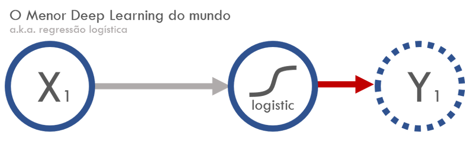
- Faz uma combinação linear inputs \(x\), adiciona um viés (bias) e depois aplica uma função de ativação não linear.
- No nosso caso, somente adiciona um parâmetro multiplicando \(x\) e um viés fixo, fazendo
\[
f(x) = w x + \text{bias}
\]
- A função de ativação é uma sigmoide, dada por
\[
\sigma(x) = \frac{1}{1 + e^{-x}}
\]
Função de custo: categorical cross-entropy
\[
\begin{aligned}
H(p, q) &= H(p) + D_{KL}(p||q) \\
&= -\sum_x p(x)\log(q(x))
\end{aligned}
\]
No nosso caso, (acho que) isso é equivalente a uma constante mais a função deviance.
Otimização
- Existem diversos algoritmos de otimização.
- Um dos mais utilizados é o de descida de gradiente estocástico.
Dados
library(tidyverse)
logistic <- function(x) 1 / (1 + exp(-x))

n <- 100000
set.seed(19910401)
dados <- tibble(
  x = runif(n, -2, 2),
  y = rbinom(n, 1, prob = logistic(-1 + 2 * x))
)
dados
## # A tibble: 100,000 x 2
##          x     y
##      <dbl> <int>
##  1 -1.19       0
##  2  0.0146     0
##  3  1.63       1
##  4 -1.51       0
##  5 -0.500      0
##  6 -0.957      1
##  7 -0.108      1
##  8  0.0595     0
##  9  1.86       1
## 10 -1.69       0
## # ... with 99,990 more rows
Ajustando uma regressão logística no R
modelo <- glm(y ~ x, data = dados, family = 'binomial')
broom::tidy(modelo)
##          term  estimate  std.error statistic p.value
## 1 (Intercept) -1.014166 0.01058750 -95.78893       0
## 2           x  2.017904 0.01216982 165.81217       0
Dúvidas
- Se é a mesma coisa, por que ele está ganhando tanta popularidade?
- Devo estudar deep learning ou posso continuar fazendo regressão logística?
CAPTCHA
library(decryptr)
model <- decryptrModels::read_model('rfb')
a <- decryptr::download_captcha("rfb", path = '.')
plot(read_captcha(a)[[1]])
decryptr(a, model)

## [1] "warabj"